Content

1. Install Python on Your Computer
   1. Install Python on Windows
   2. Install Python on Mac
   3. Install Python on Ubuntu
2. Quizzes and Answers
   • Quiz 1
   • Quiz 2

Quizzes and Answers

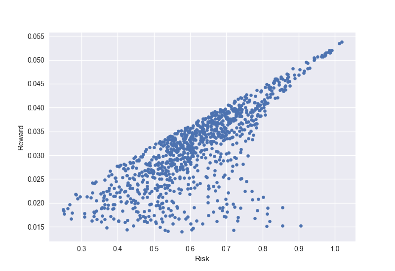
Quiz 1: Write a similar function to efficient_frontier_random_sampling in MyModule.py, but instead of printing out the risk and reward values on screen, store them in a pandas DataFrame and then use the plot.scatter (refer to documents of pandas) method of DataFrame to draw the two-dimensional risk and reward graph.

def efficient_frontier_random_sampling_df(money_spent, assets, asset_price, begin_date, end_date):
    df = []
    number_of_assets = len(assets)
    random.seed(1234)
    for counter in range(0, 1000):
        numbers = random.sample(range(1,101), number_of_assets)
        splits = np.array(numbers) / np.sum(numbers)
        daily_return = portfolio_daily_return_with_multi_assets(money_spent, assets, splits, asset_price, begin_date, end_date)
        reward = np.mean(daily_return)
        risk = np.std(daily_return)
        df.append(["portfolio{}".format(counter), risk*100, reward*100])
    df = pd.DataFrame(df, columns = ["Name", "Risk", "Reward"])
    return df

>>> reload(MyModule)
<module 'MyModule' from 'C:\\code\\MyModule.py'>

>>> ef = MyModule.efficient_frontier_random_sampling_df(1000, ["AGG", "GLD", "SPY"], AGG_GLD_SPY, "2011-01-03", "2020-12-30")
>>> ef
             Name     Risk   Reward
0      portfolio0  0.38808  0.01884
1      portfolio1  0.98768  0.05157
2      portfolio2  0.79455  0.03824
3      portfolio3  0.94300  0.04994
4      portfolio4  0.42037  0.01596
..            ...      ...      ...
995  portfolio995  0.77378  0.03913
996  portfolio996  0.34104  0.02054
997  portfolio997  0.70922  0.04050
998  portfolio998  0.53586  0.03168
999  portfolio999  0.57203  0.02205

[1000 rows x 3 columns]

>>> ef.plot.scatter("Risk", "Reward")
<AxesSubplot: xlabel='Risk', ylabel='Reward'>

>>> plt.show()

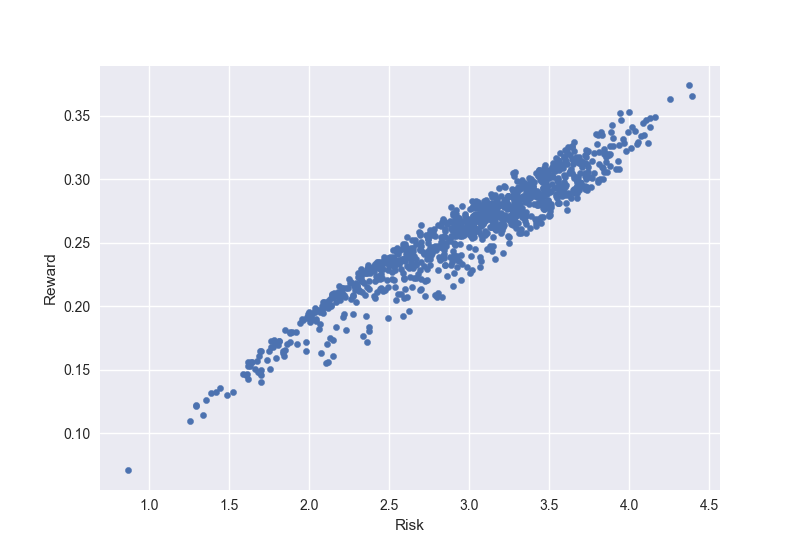
Quiz 2: Use the following five assets: TSLA, WMT, SPY, AGG, and BTC-USD, download their price data between January 3^rd, 2017 and December 30^th, 2021, and use the new function you wrote from Quiz 1 to draw the risk and reward graph.

>>> assets = [ "TSLA", "WMT", "SPY", "AGG", "BTC-USD" ]
>>> asset_prices = yfinance.download(assets, start="2017-01-03", end="2021-12-30")["Adj Close"].dropna()

[                       0%                       ]
[*******************   40%                       ]  2 of 5 completed
[*******************   40%                       ]  2 of 5 completed
[*******************   40%                       ]  2 of 5 completed
[*********************100%***********************]  5 of 5 completed

>>> ef5 = MyModule.efficient_frontier_random_sampling_df(1000,assets,asset_prices, "2017-01-03", "2021-12-30")
>>> ef5
             Name      Risk    Reward
0      portfolio0  2.702368  0.263917
1      portfolio1  2.221947  0.208947
2      portfolio2  1.355244  0.125825
3      portfolio3  3.935484  0.308334
4      portfolio4  2.157222  0.210238
..            ...       ...       ...
995  portfolio995  3.035877  0.272421
996  portfolio996  2.274952  0.209166
997  portfolio997  2.935557  0.264528
998  portfolio998  2.315283  0.212965
999  portfolio999  3.293297  0.282250

[1000 rows x 3 columns]

>>> ef5.plot.scatter("Risk", "Reward")
<AxesSubplot: xlabel='Risk', ylabel='Reward'>

>>> plt.show()